
November 9, 2012
Modeling Static Mixers, a mixer that doesn’t move may sound like an oxymoron, but it’s not. Used in various chemical species transport applications, modeling static mixers are inexpensive, accurate, and versatile. Still, there is always room for improvement. Optimizing the design of static mixers calls for computer modeling, but traditional CFD methods may not be the best way to model these mixers. What is the functioning principle of motionless mixers, and how can one simulate their performance?
How Static Mixers Work
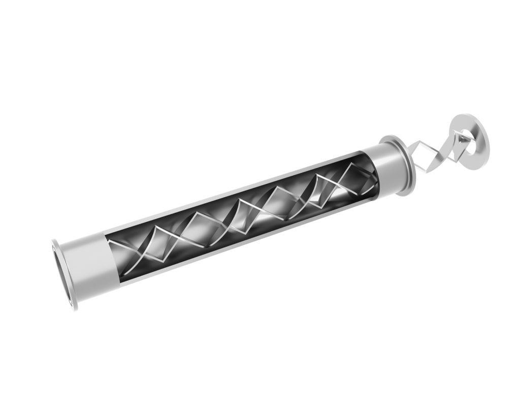
Static mixers involve pumping two streams of fluid (liquid or gas) through a pipe containing twisted blades. The different angles of the blades are what prompt the mixing of the fluid. Moreover, as the fluids travel up the tube, they interact with the blades and eventually blend. Static mixers are used in many different industries, including water treatment, petrochemical, automotive, pharmaceutical, and more.

As this type of mixing produces small losses in pressure it is a great technique for laminar flow mixing. Laminar flow exhibits low-momentum convection and high-momentum diffusion. Moreover, as opposed to turbulent flow, which is less orderly and leads to lateral mixing, laminar flow happens at lower speeds.
Modeling Laminar Mixers
In optimizing the design of a static mixer you can look at the problem in two parts. You can evaluate the mixer performance by calculating:
- The concentration’s standard deviation
- The trajectory of suspended particles through the mixer
Suppose we have a chemical species that needs to dissolve in water at room temperature. First, we will use Multiphysics and the Chemical Reaction Engineering Module to calculate the concentration’s standard deviation. Additionally, this step allows us to compute the fluid velocity and pressure as it moves through the tube from inlet to outlet. Furthermore, here you can visualize the mixing process through a series of cross-sections:
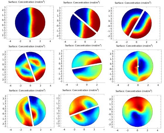
Cross-sectional plots of the concentration at different distances from the inlet of the tube.
Particle Tracing Module
In the second step, we will need to use the Particle Tracing Module to determine the particle trajectory through the tube. This is performed as a separate study, after step 1. Also, not all particles of the fluid will make it to the outlet of the tube; some will cling to the mixer walls. In addition, by running the problem in the Particle Tracing Module we can determine how many particles will be stuck inside the mixer.
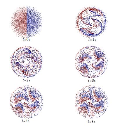
Plot of the particle position at different points in time. The red and blue particles represent two different fluids.
As mentioned earlier, traditional CFD methods may not be suitable for modeling static mixers. This is because of numerical diffusion, which does not emulate the mixing process in that the computer model shows a higher diffusivity than it does. This problem is tackled in an article on “Modeling of Laminar Flow Static Mixers” (on page 64) in the 2012 edition of COMSOL News. Here you can see how Veryst Engineering and Nordson EFD went about optimizing this type of mixer. They developed a new modeling tool for their simulations, using the CFD and Particle Tracing Modules. This case study presents an intriguing subject, so if you have an interest in improving mixer designs, I recommend reading the article.